과제1. Training a Support Vector Machine

cs231n 과제1. Training a Support Vector Machine(SVM) 정리

Training a Support Vector Machine 알고리즘

1.1 소개

알고리즘을 사용하면서 대표적인 분류 문제를 해결하기 위헤 사용하는 Loss Function Multiclass SVM loss, sotfmax classifier 두가지로 분류가 된다. 이번시간에는 SVM 사용 방법에 대한 설명이다.

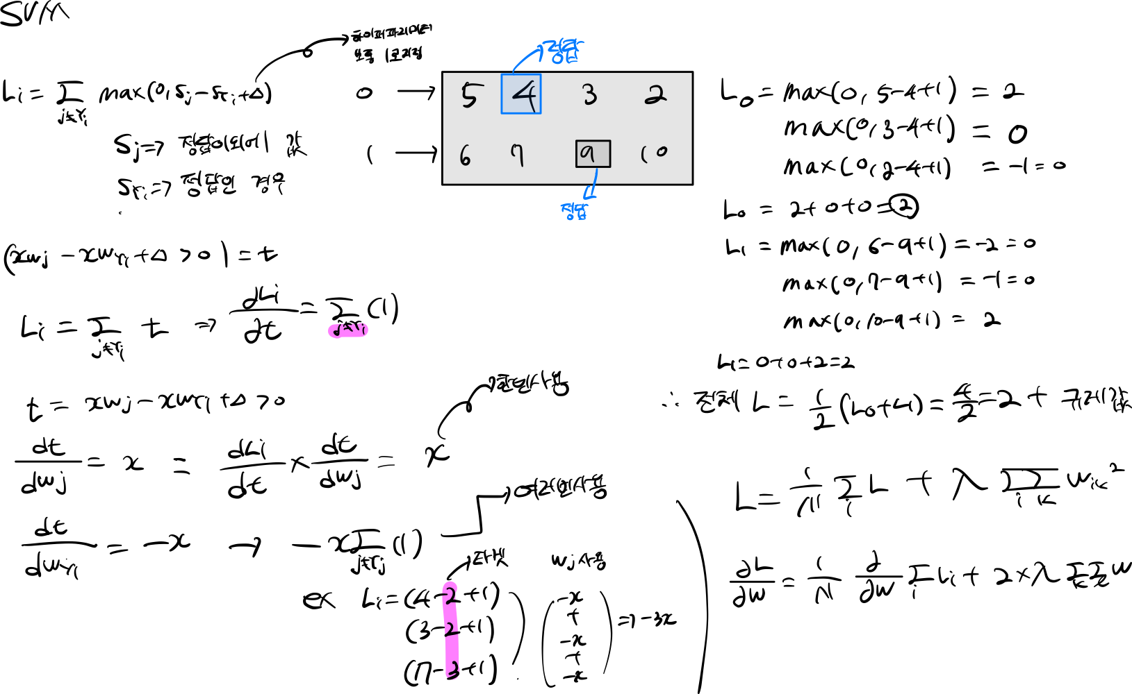
\[L_i = \sum_{j\neq y_i} \max(0, s_j - s_{y_i} + \Delta)\]

\(L_i\)는 각 데이터(rows)에 대한 손실을 의미한다.

예를 들어 \(L_i = \max(0, -7 - 13 + 10) + \max(0, 11 - 13 + 10)\)
3개의 범주를 예측하는데 13은 해당 정답에 대한 값을 의미하고, (-7, 11) 다른 정답을 예측한 값이다. (+10) 정답에 대한 마진을 조절하게 된다.

1.2 \(L\) + reg

\[L = \underbrace{ \frac{1}{N} \sum_i L_i }_\text{data loss} + \underbrace{ \lambda R(W) }_\text{regularization loss} \\\\\]

Or expanding this out in its full form:

\[L = \frac{1}{N} \sum_i \sum_{j\neq y_i} \left[ \max(0, f(x_i; W)_j - f(x_i; W)_{y_i} + \Delta) \right] + \lambda \sum_k\sum_l W_{k,l}^2\]

소개에서 봤던 \(L_i = \sum_{j\neq y_i} \max(0, s_j - s_{y_i} + \Delta)\) 수식은 각 데이터들에 대한 손실도 였기 때문에 전체 데이터 손실을 구해야한다.

데이터 손실 부분을 먼저 구하고 \(\underbrace{ \frac{1}{N} \sum_i L_i }_\text{data loss}\)

규제에 대한 손실값도 추가해야한다.\(\underbrace{ \lambda R(W) }_\text{regularization loss}\)

규제 방식은 이전에 사용했던 L2 규제를 사용하기 때문에 모든 가중치에 제곱하고 더한다\(\lambda \sum_k\sum_l W_{k,l}^2\)

2. train

2.1 svm loss naive

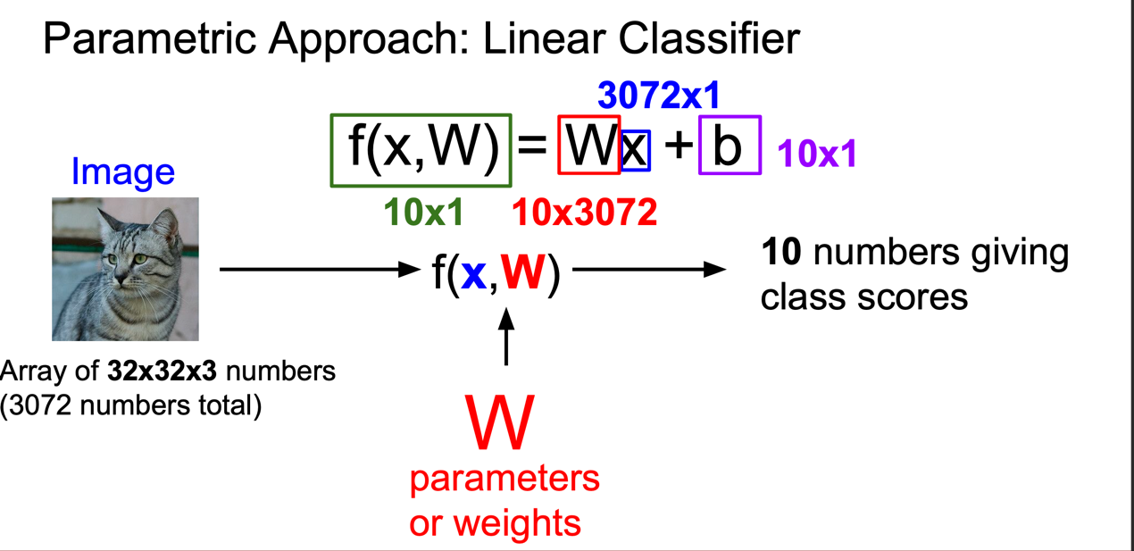
먼저 linear classifier \(W * x + b\) 사용해 class scores 설정해야한다.

각각 파아미터는 \(W\), \(x\), \(b\) 파리미터롤 사용이 될것이다.

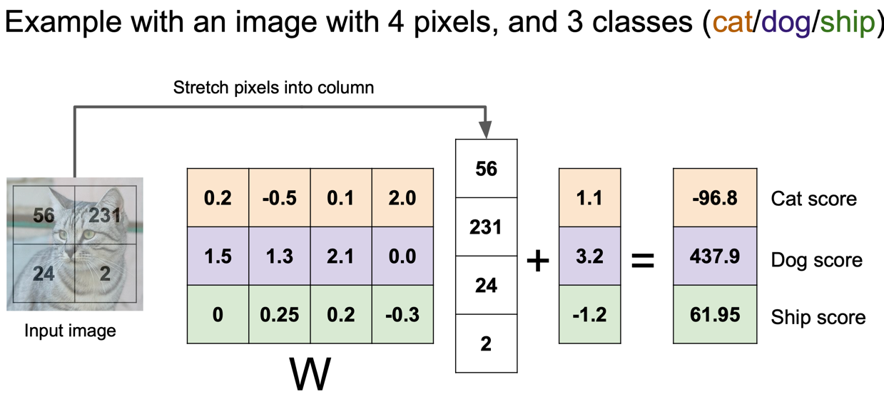
최종 적인 class scores 받는 그림이다.
이제 최적에 값을 찾아 가기위해서 Loss function 사용해 W 값을 업데이트 시킨다.

W 값에 최적에 값을 찾아가는 방식은 경사하강법을 사용하게된다. (미분한다!)

    dW = np.zeros(W.shape)  # initialize the gradient as zero

    # compute the loss and the gradient
    num_classes = W.shape[1]
    num_train = X.shape[0]
    loss = 0.0
    for i in range(num_train):
        scores = X[i].dot(W)
        correct_class_score = scores[y[i]]
        for j in range(num_classes):
            if j == y[i]:
                continue

            margin = scores[j] - correct_class_score + 1  # note delta = 1
            if margin > 0:
                loss += margin

                dW[:, y[i]] = dW[:, y[i]]  - X[i]

                dW[:, j] = dW[:, j] + X[i]

    # Right now the loss is a sum over all training examples, but we want it
    # to be an average instead so we divide by num_train.
    loss /= num_train

    # Add regularization to the loss.
    loss += reg * np.sum(W * W)

    #############################################################################
    # TODO:                                                                     #
    # Compute the gradient of the loss function and store it dW.                #
    # Rather that first computing the loss and then computing the derivative,   #
    # it may be simpler to compute the derivative at the same time that the     #
    # loss is being computed. As a result you may need to modify some of the    #
    # code above to compute the gradient.                                       #
    #############################################################################
    # *****START OF YOUR CODE (DO NOT DELETE/MODIFY THIS LINE)*****
    dW /= num_train

    dW += 2*W*reg

• scores = X[i].dot(W) : 내적을 사용해 class socres 받아 드린다.
• correct_class_score = scores[y[i]] : SVM Loss function 알고리즘에 따라 해당 데이터에 정답 score 뽑아내야한다.
• classes 종류 만큼 반복문을 실행해야한다.
• 민약 정답과 for 돌린 값이 일치하다면 그 값은 계산하면 안된다
• margin = scores[j] - correct_class_score + 1 # note delta = 1 : margin 계산하고 값이 0이상일 때에 loss 추가한다.
• margin > 0 이상이면 dW 업데이트 시켜준다.
• loss /= num_train 훈련 데이트 만큼 값을 나눠야한다. 규제 또한 추가해야한다.
• dW 미분하기 때문에 값을 추가해야한다.

2.2 svm loss vectorized

2.1 에서는 수식적인 부분으로 접근 했다면, 이번 챕터에서는 기하학적인 관점에서 접근할 것이다.

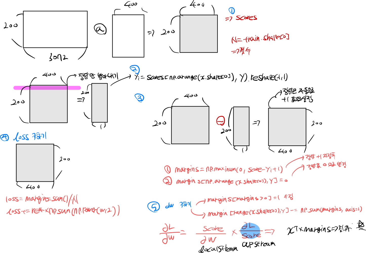
    score = X.dot(W)
    yi = score[np.arange(X.shape[0]), y].reshape(-1, 1)

    margins = np.maximum(0, score - yi + 1)
    margins[np.arange(X.shape[0]), y] = 0

    loss = margins.sum() / X.shape[0]
    loss += reg * np.sum(np.power(W, 2))

    # *****END OF YOUR CODE (DO NOT DELETE/MODIFY THIS LINE)*****

    #############################################################################
    # TODO:                                                                     #
    # Implement a vectorized version of the gradient for the structured SVM     #
    # loss, storing the result in dW.                                           #
    #                                                                           #
    # Hint: Instead of computing the gradient from scratch, it may be easier    #
    # to reuse some of the intermediate values that you used to compute the     #
    # loss.                                                                     #
    #############################################################################
    # *****START OF YOUR CODE (DO NOT DELETE/MODIFY THIS LINE)*****

    margins[margins > 0] = 1
    margins[range(X.shape[0]), y] -= np.sum(margins, axis=1)

    dW = (X.T).dot(margins) / X.shape[0]
    dW = dW + reg * 2 * W

• score = X.dot(W) : 내적을 통해 값을 구한다.
• yi = score[np.arange(X.shape[0]), y].reshape(-1, 1) : 정답만 뽑아낸다.
• margins = np.maximum(0, score - yi + 1) : 한 번에 loss 값을 계산한다(정답 값은 + 마진만큼 증가)
• margins[np.arange(X.shape[0]), y] = 0 : 정답 값을 0으로 초기화 한다.
• loss = margins.sum() / X.shape[0] : loss 값을 계산한다.
• loss += reg * np.sum(np.power(W, 2)) : 규제 추가한다.
• margins[margins > 0] = 1 : margin 값이 0 이상이면 모드 1로 초기화한다.
• margins[range(X.shape[0]), y] -= np.sum(margins, axis=1) : 0이 있는 만큼 정답 데이터에 1을 빼준다 (0이 있는 만큼갯수 -1 증가)
• dW = (X.T).dot(margins) / X.shape[0] : 값을 내적한다.
• dW = dW + reg * 2 * W : 규제 또한 미분을 해야한다.

참조

• https://cs231n.github.io/