과제2. Batch Normalization
배치 정규화 코드 구현
1. Introduce
신경망을 학습하는데 문제점을 흔하게 발생하는 문제점이 Vanishing, Exploding 발생한다.
잘 사용하지 않지만, 설명하기 좋은 Relu 함수를 가지고 설명을 한다면
Relu 값은 음수로 값이 가게 된다면 모든 값이 0이 된다. 그 상태로 backpropagation 실행한다면,
\(dw = X * \frac{dLoss}{dv}\) X 값들은 모두 0이 될것이다. 그럼 역전파가 제대로 발생하지 않을 것이다.
반대로 Exploding 값이 된다면
\(dw = X * \frac{dLoss}{dv}\) X 큰값을 가지기 때문에 값이 폭팔하게 될것이다.
이것을 해결하기 가중치를 적절하게 초기화 해야하지만, 결국 layer 지날수록 값들은 0으로 수렴하게 될것이다. (Xavier 초기화 또는 He 초기화 한다면 문제를 그나마 해결할 수 있음)
그래서 해결 방법으로 Batch Normalization 논문이 나오게 되었다.
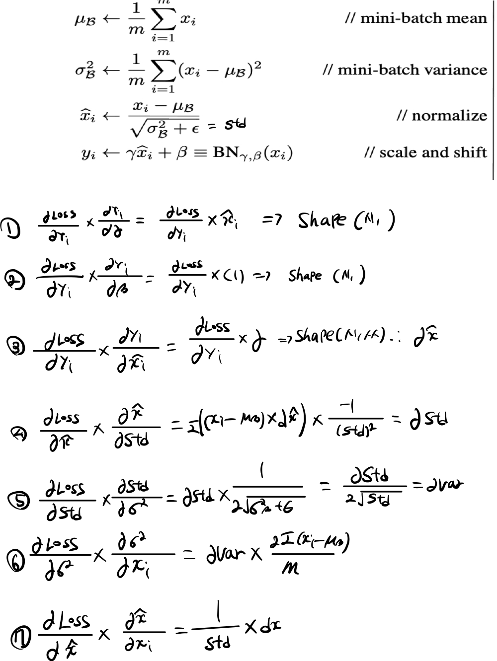
Batch Normalization 사용방법은 아래와 같은 계산법을 사용하게 된다.
\(\begin{align}
& \mu=\frac{1}{N}\sum_{k=1}^N x_k & v=\frac{1}{N}\sum_{k=1}^N (x_k-\mu)^2 \\
& \sigma=\sqrt{v+\epsilon} & y_i=\frac{x_i-\mu}{\sigma} \\
& y_i = \gamma*y_i + \beta
\end{align}\)
2. Batch Norm Forward
2.1 forward 과정
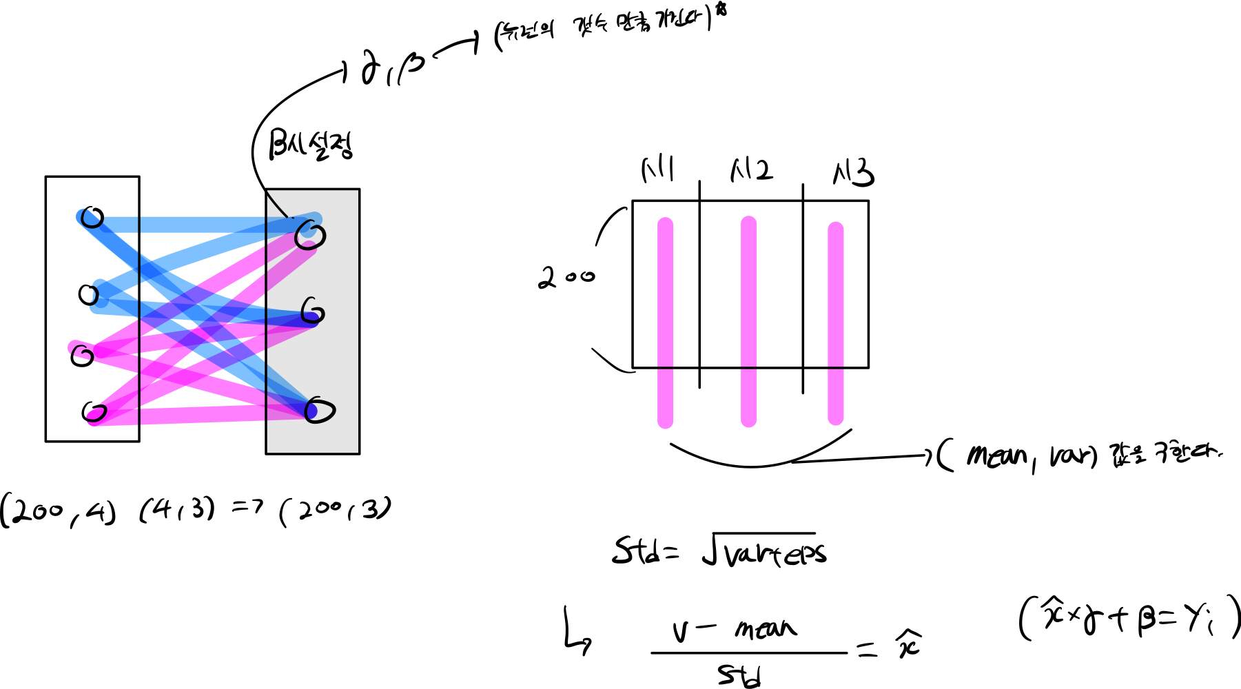
2.1.1 원리
- 뉴런당 해당하는 평균 값을 구한다.
- 분산을 구하고
- 표준편차 =분산 + eps 구한다.
- 정규분포를 구해
- gamma, beta 추가해준다.
2.1.2 code
def batchnorm_forward(x, gamma, beta, bn_param):

    mode = bn_param["mode"]
    eps = bn_param.get("eps", 1e-5)
    momentum = bn_param.get("momentum", 0.9)

    N, D = x.shape
    running_mean = bn_param.get("running_mean", np.zeros(D, dtype=x.dtype))
    running_var = bn_param.get("running_var", np.zeros(D, dtype=x.dtype))

    out, cache = None, None
    if mode == "train":

        x_mean = np.mean(x, axis=0)
        var = np.var(x, axis=0)

        std = np.sqrt(var + eps)
        x_hat = (x - x_mean) / std
        out = gamma * x_hat + beta

        shape = bn_param.get('shape', (N, D))
        axis = bn_param.get('axis', 0)

        cache = x, x_mean, var, std, gamma, x_hat, shape, axis # save for backprop

        if axis == 0:
            running_mean = momentum * running_mean + (1 - momentum) * x_mean # update overall mean
            running_var = momentum * running_var + (1 - momentum) * var  # update overall variance

    elif mode == "test":
        x_hat = (x - running_mean) / np.sqrt(running_var + eps)
        out = gamma * x_hat + beta

    else:
        raise ValueError('Invalid forward batchnorm mode "%s"' % mode)

    bn_param["running_mean"] = running_mean
    bn_param["running_var"] = running_var

    return out, cache
2.2 backward 과정
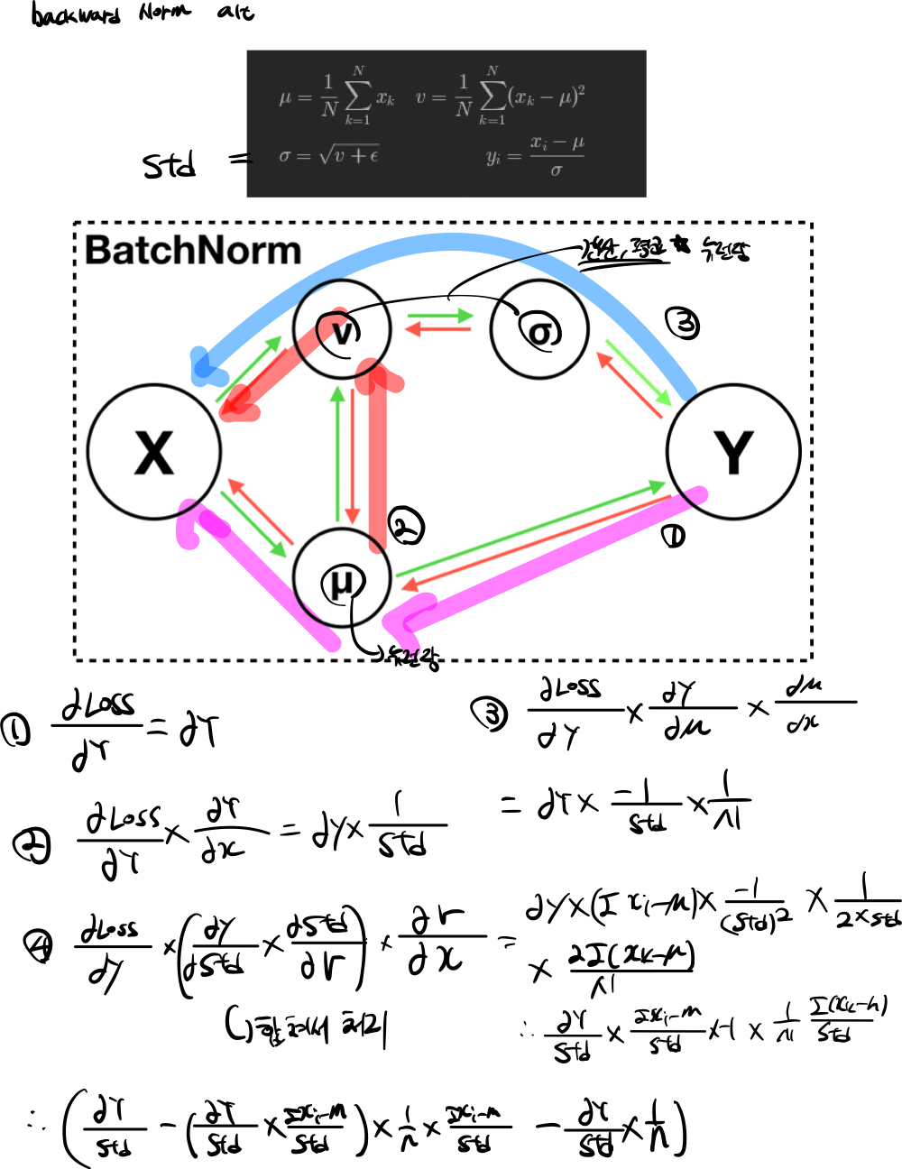
2.2.1 원리
밑에 그림은 backpropagation 진행하는 과정을 표시했다.

2.2.2 code
def batchnorm_backward(dout, cache):
    x, mu, var, std, gamma, x_hat, shape, axis = cache

    dbeta = dout.sum(axis=0)

    dgamma = (dout * x_hat).sum(axis=0)

    dx_hat = dou t * gamma

    dstd = -np.sum(dx_hat * (x-mu), axis=0) / (std**2)

    dvar = 0.5 * dstd / std

    dx_1 = dx_hat / std

    dx_2 = 2 * (x - mu) * dvar / len(dout)

    dx_k1 = dx_1 + dx_2

    dmu = -np.sum(dx_k1, axis=0)  # derivative w.t.r. mu

    dx_k2 = dmu / len(dout)  # partial derivative w.t.r. dx

    dx = dx_k1 + dx_k2

    return dx, dgamma, dbeta
2.2.3 backnorm alt

def batchnorm_backward_alt(dout, cache):
    dx, dgamma, dbeta = None, None, None

    _, _, _, std, gamma, x_hat, shape, axis = cache  # expand cache

    dbeta = dout.sum(axis=axis)
    dgamma = (dout * x_hat).sum(axis=axis)

    dx_hat = dout * gamma
    N = len(dout)

    dx = dx_hat / std

    dx = dx - (((dx * x_hat).sum(axis=0) * x_hat) / N) - (dx.sum(axis=0) / N)

    return dx, dgamma, dbeta
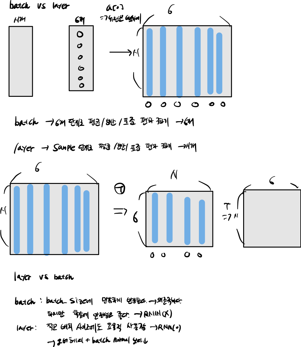
3 layer-normal
그래서 나온 방법이 layer-normal 방식이다.
layer-normal 방식은 layer 기준으로 평균과 분산을 구하게 된다. 즉 batch-normal 반대되는 성질을 가지고 있다.
4. Question
4.1 Question 1
Describe the results of this experiment. How does the weight initialization scale affect models with/without batch normalization differently, and why?
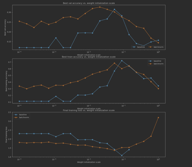
4.1.2 Answer 1
정확도
- 전체적인 정확도를 살펴보면 정규화 했을시 더 좋은 정확도를 나타내고 있다.
- 왜냐하면 가중치가 너무 작거나, 너무작거나, 너무 크면 vanishing, Exploding 문제가 발생한다.
- 예를 들어 가중치 값이 너무 작으면, backpropagation dx = local grad(x) * upstream(미분값) 하게된다면, w값이 작기 때문에 모든 활성화 함수는 0으로 갈것이다.
- 문제를 해결하는 방식으로 BN을 사용해서 모든 뉴런에 들어가는 값을 정규분포르 변경하여 값들을 정규화 시킨다.
- 위에 그럼에 보이는 것처럼 가중치가 너무 작더라고 BN을 사용했기 때문에 정확도가 올라간것을 볼 수 있고, 반대로 BN 사용하지 않은 경우는 기울기 손실로 값들잉 좋은 정확도를 볼 일수없다.
- 가중치가 너무 작으면 모든 확설화 함수 값은 0으로 가고, 반대로 너무 크면 기울기가 죽는 현상이 발생한다.
스케일 조정
- 현재 가중치 10^-1 부분을 보면 특이한 지점을 볼 수 있다.
- 10^-1 부분이 최적에 가중치 값을 찾았다고 볼 수 있다. 하지만 그 이후 높아진다면, 기울기 손실이 발생하기 때문에 조절해야한다.
4.2 Question 2
Describe the results of this experiment. What does this imply about the relationship between batch normalization and batch size? Why is this relationship observed?
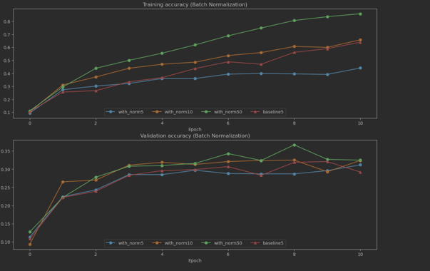
4.2.2 Answer 2
- 배치 사이즈가 더 많아 진다는 것은 표본이 더 많이 생긴다는 뜻이다.
- 만약 배치 사이즈가 한개 밖에 안된다면, 위에 공식에 따르면 단일 뉴런만 받아진다.
- 그럼 배치 사이즈가 크면 클수록 집단에 사이즈가 커진다는 것을 알수있다
4.3 Question 3
Which of these data preprocessing steps is analogous to batch normalization, and which is analogous to layer normalization?
- Scaling each image in the dataset, so that the RGB channels for each row of pixels within an image sums up to 1.
- Scaling each image in the dataset, so that the RGB channels for all pixels within an image sums up to 1.
- Subtracting the mean image of the dataset from each image in the dataset.
- Setting all RGB values to either 0 or 1 depending on a given threshold.
4.3.2 Answer:
- 2번은 layer-norm 대한 이야기 이다. layer는 전체 픽셀의 값을 이용하여 평균, 분산을 구하게 된다.
- 3번은 batch-norm 대한 이야기 이다. 각각에 dataset 기준으로 평균, 분산을 구한다음에 새로운 값을 구한다.
4.4 Question 3
When is layer normalization likely to not work well, and why?
- Using it in a very deep network
- Having a very small dimension of features
- Having a high regularization term
4.3.3 Answer:
- 2,3 정답
- 차원이 적을 수 록 정규화할 표본들아 적아진다.
Additional references
- https://cs231n.github.io