과제2. Fully-Connected-Nets

다층 신경망 로직 구현

1. introduce

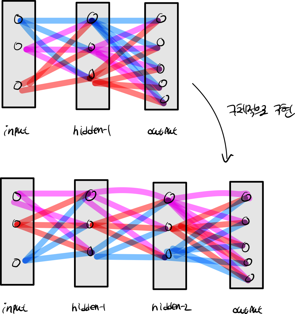
과제 1번에서는 쉽게 hidden-layer 한 개만 있을 경우 구현을 완료했습니다. 하지만 신경망은 여러개로 존재다.

심층 신경망을 구체적으로 구현하는 과정을 걸치게 됩니다.

2. init

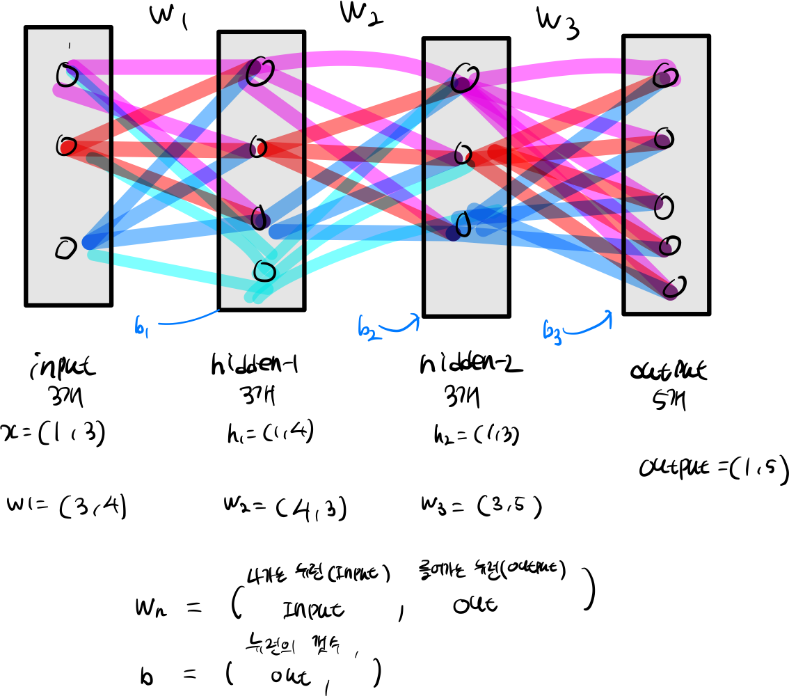
네트워크를 구성하게 된다면 첫번째 신경망에서 할 일은 파라미터값을 정의 해야한다.
파라미터는 weight, bias 등 네트워크에 기본이 되는 값들을 설정해야 한다.

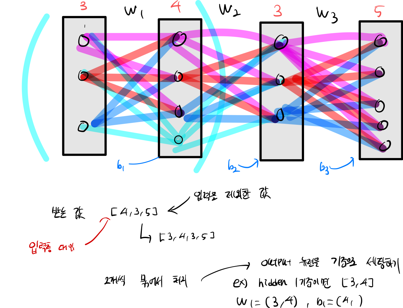
        hidden_dim_layer = copy.deepcopy(hidden_dims)

        hidden_dim_layer.insert(0, input_dim)
        hidden_dim_layer.append(num_classes)
        for index in range(1,len(hidden_dim_layer)):
            self.params[f"W{index}"] = np.random.randn(hidden_dim_layer[index -1], hidden_dim_layer[index]) * weight_scale
            self.params[f"b{index}"] = np.zeros((1, hidden_dim_layer[index]))

out layer 기준으로 가중치, bias를 효율적으로 초기화를 해야한다.
input layer 기준으로 한다면, input 기준으로 한다면, bias 설정에서 for 문안에서 if 작성으로 분기를 나눠야한다.

3. train

        cache_list = []
        input_list = [0, X]

        for index in range(1, self.num_layers +1):
            keys = [f'W{index}', f'b{index}', f'gamma{index}', f'beta{index}']
            w, b, gamma, beta = (self.params.get(k, None) for k in keys)  # get param vals
            bn = self.bn_params[index -1] if gamma is not None else None
            do = self.dropout_param if self.use_dropout else None

            if index == self.num_layers:
                fc, cache = affine_forward(input_list[index], self.params[f'W{index}'], self.params[f'b{index}'])
            else:
                fc, cache = affine_normally_forward(input_list[index], w, b, gamma, beta, bn,
                                                    bn_type=self.normalization, do=do)

            input_list.append(fc)
            cache_list.append(cache)

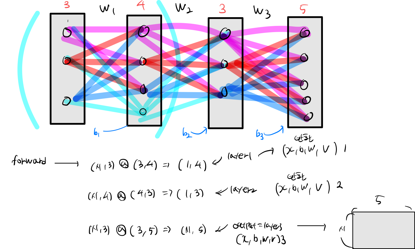
forward 하는 방식링크 클릭하면 이전에 설명했던 블로그 내용 나옵니다!

4. loss

        loss, dz = softmax_loss(scores, y)
        weight = 0

        for index in range(self.num_layers, 0, -1):
            weight = (self.params[f'W{index}'] * self.params[f'W{index}']).sum()
            do = self.dropout_param if self.use_dropout else None
            if index == self.num_layers:
                dz, grads[f'W{index}'], grads[f'b{index}'] = affine_backward(dz, cache_list[index -1])
            else:
                dz, grads[f'W{index}'], grads[f'b{index}'], gamma, beta = affine_batchnoral_relu_backward(dz, cache_list[index - 1],  bn_type=self.normalization)

                if gamma is not None and beta  is not None :
                    grads[f'gamma{index}'], grads[f'beta{index}']= gamma, beta
            grads[f'W{index}'] += self.reg * self.params[f'W{index}']

        loss += 0.5 * self.reg * weight

backward 하는 방식링크 클릭하면 이전에 설명했던 블로그 내용 나옵니다!

5. optimizer

5.1 SGD

GD를 사용하지만, 데이터를 전체를 GD 하는 것이 아니라, 미니배치를 사용해 경사하강법을 실행한다.

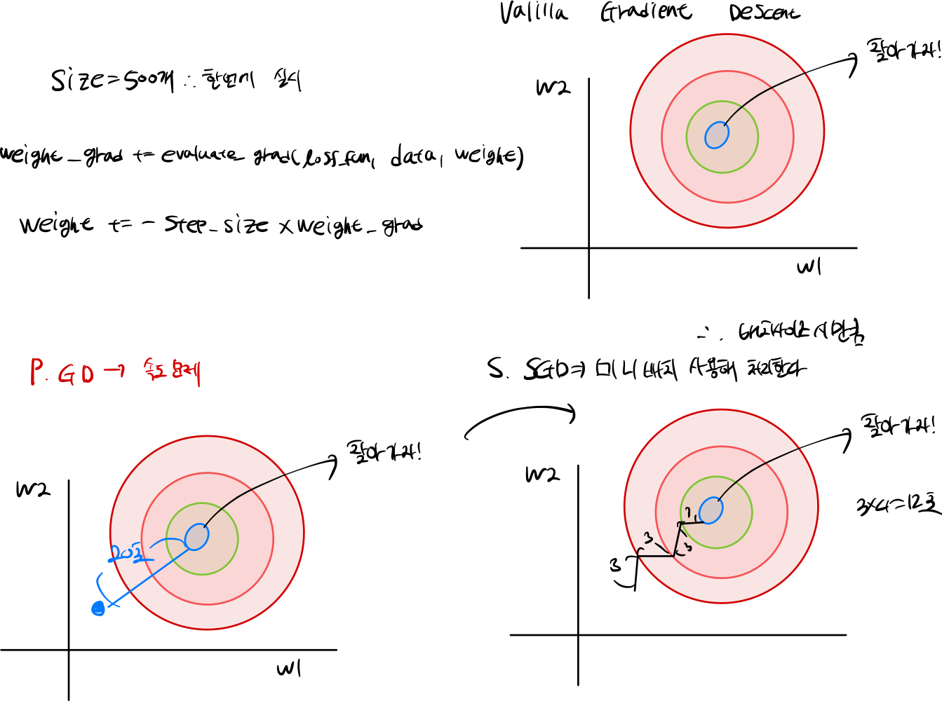
5.1.1 SGD 문제점

• saddle point & Local minima을 유발시킨다.
• Saddle point는 기울기가 0인 지점에서는 더 이상 업데이트를 실행하지 않습니다.
• Local minima 지역적인 최솟값을 Grobal 극소로 착각할 수 있다.

5.1.2 code

def sgd(w, dw, config=None):
    """
    Performs vanilla stochastic gradient descent.

    config format:
    - learning_rate: Scalar learning rate.
    """
    if config is None:
        config = {}
    config.setdefault("learning_rate", 1e-2)

    w -= config["learning_rate"] * dw
    return w, config

5.2 SGD + Momentum

문제를 해결하기 위해 일정 한 가속도를 설정해 값이 zero 머물지 않도록 설정하게 됩니다.

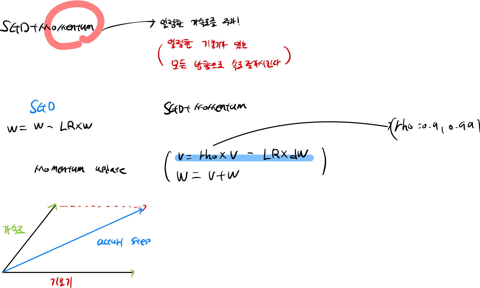
5.2.1 Momentum 문제점

가속도를 지정하기 때문에 멈추어야 할 시점에서도 가속력 때문에 휠신 멀리 간다는 단점이 있습니다.
단순 해결 방법는 rho 값은 마찰계수를 강하게 지정하게 됩니다

5.2.2 code

def sgd_momentum(w, dw, config=None):
    if config is None:
        config = {}
    config.setdefault("learning_rate", 1e-2)
    config.setdefault("momentum", 0.9)
    v = config.get("velocity", np.zeros_like(w))


    next_w = None

    v = config['momentum'] * v - config['learning_rate'] * dw
    next_w = w + v

    config["velocity"] = v

    return next_w, config

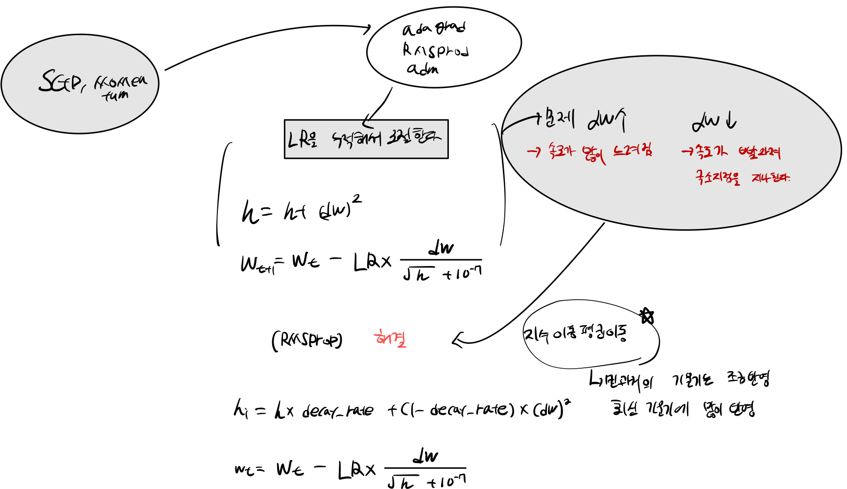
5.3 RMSprop

adagrad 나온 문제점으로 Adagrad는 과거의 기울기를 제곱하여 더하는 학습 방식으로 진행할 수 록 점점 갱신 강도가 약해진다.
이를 개선한 방식이 RMSProp 방식으로 과거의 기울기들을 똑같이 더해나가는 것이 아니라, 먼과거의 기울기는 조금 반영하고 최신의 기울기는 많이 반영한다. (지수 이동 평균 원리 사용)

5.3.1 code

def rmsprop(w, dw, config=None):

    if config is None:
        config = {}
    config.setdefault("learning_rate", 1e-2)
    config.setdefault("decay_rate", 0.99)
    config.setdefault("epsilon", 1e-8)
    config.setdefault("cache", np.zeros_like(w))

    next_w = None

    config['cache'] = config['cache'] * config['decay_rate'] + (1 - config['decay_rate']) * dw ** 2
    next_w = w - config['learning_rate'] * dw / (np.sqrt(config['cache']) + config['epsilon'])


    return next_w, config

5.4 Adam

Adam 사용되는 원리는 Momentum + RMSProp 합친 형태로 기울기 가속도를 주고 LR 누적하여 최적화를 실행하게 된다.

5.4.1 code

def adam(w, dw, config=None):
    if config is None:
        config = {}
    config.setdefault("learning_rate", 1e-3)
    config.setdefault("beta1", 0.9)
    config.setdefault("beta2", 0.999)
    config.setdefault("epsilon", 1e-8)
    config.setdefault("m", np.zeros_like(w))
    config.setdefault("v", np.zeros_like(w))
    config.setdefault("t", 0)

    next_w = None
    keys = ['learning_rate','beta1','beta2','epsilon','m','v','t']
    lr, beta1, beta2, eps, m, v, t = (config.get(k) for k in keys) 

    config['t'] = t = t + 1
    config['m'] = m = beta1 * m + (1 - beta1) * dw
    mt = m / (1 - beta1**t)
    config['v'] = v = beta2 * v + (1 - beta2) * (dw**2)
    vt = v / (1 - beta2**t)
    next_w = w - lr * mt / (np.sqrt(vt) + eps)

    return next_w, config

Question

5.1 Question 1

Inline Question 1: Did you notice anything about the comparative difficulty of training the three-layer network vs. training the five-layer network? In particular, based on your experience, which network seemed more sensitive to the initialization scale? Why do you think that is the case?

Answer : 만약 신경망의 계층이 더 깊다면, 많은 가중치를 학습시켜야 합니다. 이것은 계층이 많아질수록 과적합과 관련이 될 수 있습니다. 계층이 많아지면 그만큼 모델이 더 복잡해지며, 훈련 데이터에 과도하게 적합하려는 경향이 있습니다.

가중치 초기값이 작은 값으로 설정되면, 얕은 신경망 (예: 3 계층)의 경우에는 순전파(forward propagation)가 원할하게 진행되고 출력 레이어까지 문제 없이 정보가 전달될 수 있습니다. 그러나 계층이 깊어질수록 작은 초기값을 곱하게 되면 가중치 값들이 0으로 수렴하는 경향이 있습니다. 이것은 그보다 더 깊은 계층이 가중치에 민감하게 반응하게 됨을 의미합니다.

따라서, 신경망의 깊이가 증가할 때 가중치 초기값을 적절하게 설정하는 것이 중요합니다. 일반적으로 Xavier 초기화 또는 He 초기화와 같은 초기화 기법을 사용하여 가중치를 적절하게 설정하고, 그로 인해 그래디언트 소실 또는 폭발 문제를 완화할 수 있습니다. 이렇게 하면 심층 신경망에서도 효과적인 학습이 가능하며, 과적합을 줄이고 모델의 성능을 개선할 수 있습니다.

5.1 Question 2

Inline Question 2:

AdaGrad, like Adam, is a per-parameter optimization method that uses the following update rule:

cache += dw**2
w += - learning_rate * dw / (np.sqrt(cache) + eps)

John notices that when he was training a network with AdaGrad that the updates became very small, and that his network was learning slowly. Using your knowledge of the AdaGrad update rule, why do you think the updates would become very small? Would Adam have the same issue?

Answer : 신경망에서 학습률(LR) 설정은 매우 중요합니다. 학습률을 적절하게 설정하기 위해 LR 감소(LR decay) 기술을 사용하게 됩니다. 이 기술은 학습 단계마다 매개변수에 맞게 학습률을 조절하여 최적화된 LR을 설정합니다.

한편, AdaGrad 방식은 이전에 계산된 기울기를 제곱하여 루트를 씌우고 현재 기울기로 나누는 방식으로 학습률을 조절합니다. 이로 인해 이전에 큰 기울기를 가진 매개변수는 학습 속도가 느려지고, 작은 기울기를 가진 매개변수는 학습 속도가 빨라집니다.

그러나 AdaGrad 방식은 과거 기울기의 누적 제곱값으로 인해 학습이 느려질 수 있습니다. 이를 해결하기 위해 RMSProp 방식을 도입합니다. RMSProp은 과거 기울기의 누적을 감소시키고 최신 기울기에 더 많은 가중치를 부여하여 학습률을 더 잘 조절합니다.

더 나아가, RMSProp과 모멘텀(Momentum)을 결합한 방식으로 Adam이 등장합니다. Adam은 최신 기울기와 모멘텀을 활용하여 더욱 효과적인 학습률을 설정하며, 이를 통해 빠른 수렴과 안정적인 학습을 가능하게 합니다.